LIBOR Interest Rates Analysis
- Introduction
- Extract and visualize raw data
- Term structure
- Non-stationary vs. stationary time series
Introduction
LIBOR, which stands for London Interbank Offered Rate, is the average interbank interest rate at which a selection of banks on the London money market are prepared to lend to one another. LIBOR comes in 7 maturities (from overnight to 12 months) and in 5 different currencies including the US dollar, the euro, the British pound, the Japanese yen, and the Swiss franc. The official LIBOR interest rates are announced once per working day at around 11:45 a.m.
LIBOR is also the basis for consumer loans in countries around the world, so it impacts consumers just as much as it does financial institutions. The interest rates on various financial products such as credit cards, car loans, and adjustable rate mortgages fluctuate based on the LIBOR rate. This change in rate helps determine the ease of borrowing between banks and consumers.
In this project I will present some statistical analysis on the LIBOR interest rates for various USD maturities obtained from FRED website.
Extract and visualize data
Here is the list of libraries that I will be using for this project:
library(quantmod)
library(tidyr)
library(ggplot2)
library(corrplot)
library(fitdistrplus)
library(ggpubr)
library(VarianceGamma)
library(factoextra)
require(gridExtra)
In order to get the LIBOR IR, I defined a function that requires the ticker of the maturity from FRED website and the date range.
setDefaults(getSymbols, src="FRED")
"getSymbols.warning4.0"=FALSE
get_data <- function(ticker,date_range)
{
  t=getSymbols(as.character(ticker), env=.GlobalEnv, auto.assign = F)
  t=t[date_range]
  colnames(t) <- c("IR")  # change col name
  sum(is.na(t$IR))        # count the number of NA
  t= t[!is.na(t),]        # remove the NA rows
  return (t)
}
### For this example I will be using data from 1986 to 2019
date_range='199801/201112'

USDON=get_data("USDONTD156N", date_range)
USD1M=get_data("USD1MTD156N", date_range)
USD3M=get_data("USD3MTD156N", date_range)
USD6M=get_data("USD6MTD156N", date_range)
USD9M=get_data("USD9MTD156N", date_range)
USD12M=get_data("USD12MD156N", date_range)
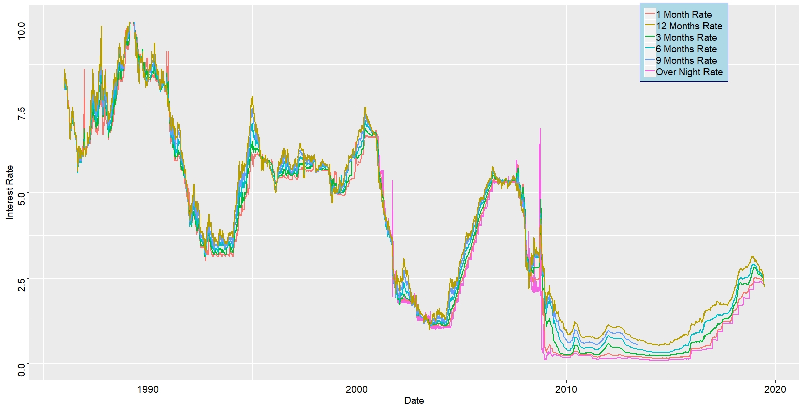
Here is the graph for USD LIBOR Interest Rates for different maturities:
A=ggplot() +
  geom_line(data = USDON, aes(x=index(USDON), y=USDON, col="Over Night Rate"),size=1)+
  geom_line(data = USD1M, aes(x=index(USD1M), y=USD1M, col="1 Month Rate"),size=1)+
  geom_line(data = USD3M, aes(x=index(USD3M), y=USD3M, col="3 Months Rate"), size=1)+
  geom_line(data = USD6M, aes(x=index(USD6M), y=USD6M, col="6 Months Rate"), size=1)+
  geom_line(data = USD9M, aes(x=index(USD9M), y=USD9M, col="9 Months Rate"), size=1)+
  geom_line(data = USD12M, aes(x=index(USD12M), y=USD12M, col="12 Months Rate"),size=1)+
  ylab("Interest Rate")+
  xlab("Date")+ylim(0, 10)+
  theme_gray(base_size = 14)+
  theme(axis.text.y = element_text(size=14, angle = 90 , colour = "black"))+
  theme(axis.text.x = element_text(size=14, colour = 'black'))+
  theme(legend.position = c(0.85, 0.9))+
  theme(legend.background = element_rect(fill="lightblue", linetype="solid", colour ="darkblue"))+
  theme(legend.title=element_blank())+
  theme(legend.text=element_text(size=14))
windows()
print(A)

As you can see there is cycle of up and down in the LIBOR interest rates over the last 3 and half decades presented in the graph above. The cycle usually happens every decade. The stock markter crach, on what become known as Black Monday, took place in 1987. Global stock markets crashed, including in the US, where the Dow Jones index lost 508 points or 23% of its value.
In 1994 a sudden devaluation of the Mexican peso triggered what would become known as the Tequila crisis, which would become a massive interest rate crisis and result in a bond rout. Analysts regard the crisis as being triggered by a reversal in economic policy in Mexico, whereby the new president, Ernesto Zedillo, removed the tight currency controls his predecessor had put in place. While the controls had established a degree of market stability, they had also put an enormous strain on Mexico’s finances. Prior to Zedillo, banks had been lending large amounts of money at very low rates. With a rebellion in the poor southern state of Chiapas adding to Mexico’s risk premium, the peso’s value fell by nearly 50% in one week.
In 1999-2000 was the dotcom bubble, which was preceded by a bull rush into technology and interenet related stocks. Individuals became millionaires overnight through companies such as eBay and Amazon. Followed by that, was the financial crisis of 2007-2009 that was the most-severe financial crisis since the Great Depression, and it wreaked havoc in financial markets around the world. Triggered by the collapse of the housing bubble in the U.S., the crisis resulted in the collapse of Lehman Brothers (one of the biggest investment banks in the world), brought many key financial institutions and businesses to the brink of collapse, and required government bailouts of unprecedented proportions. It took almost a decade for things to return to normal, wiping away millions of jobs and billions of dollars of income along the way.
Term Structure
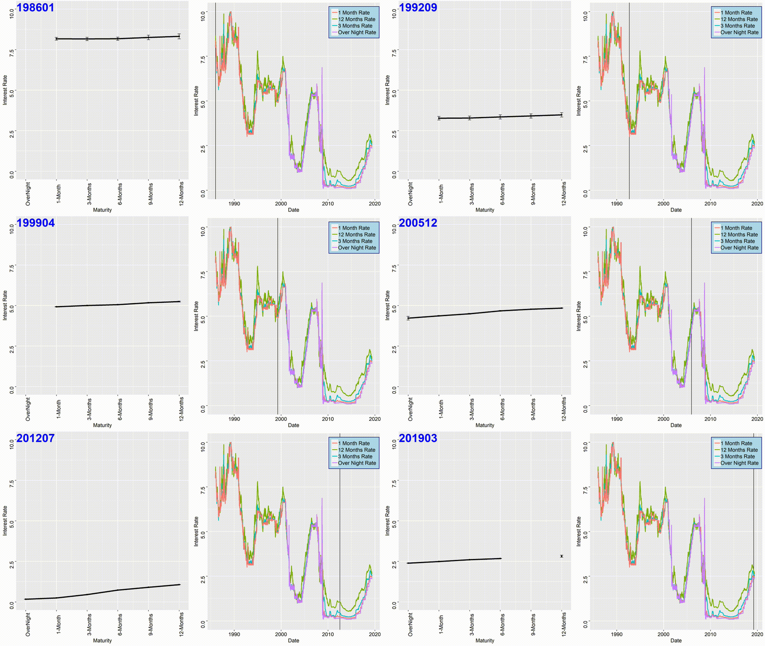
Term structure of interest rates is the relationship between interest rates and different maturities. The term structure reflects expectations of market participants about future changes in interest rates. The term structure graph can have three different outcomes as depicted in the figure below. If there is a highly positive normal curve, it is a signal investors believe future economic growth to be strong and inflation high. If there is a highly negative inverted curve, it is a signal investors believe future economic growth to be sluggish and inflation low. A flat yield curve means investors are unsure about the future.

In this section I will show how to get the term structure for USD LIBOR rates as illustrated in the top figure of this page. It would be time consuming to plot the term structure for every single day. Therefore, for this project I have manupilated the data to get the term structure for every month of the year. That means, we have to aggregate the data for every month of the year and get the mean and standard deviation:
### USD Over night:
# extract the index (date)
USDON_f=fortify(USDON)
# since we want to aggregate the data by month and take the average, we will only store the year and month into a new column
USDON_f[,3] <- as.factor(format(as.Date(USDON_f$Index, format="%Y/%m/%d"),"%Y%m"))
# calculate the mean for each month
USDON_mean <- aggregate(USDON_f$IR,by=list(USDON_f$V3),FUN=mean)
# calculate the standard deviation for each month
USDON_sd<- aggregate(USDON_f$IR,by=list(USDON_f$V3),FUN=sd)
#combine the two data together
USDON_mean=cbind(USDON_mean, USDON_sd[,2])
# create a new column with the maturity name --- we will need it later
USDON_mean[,4]="USDON"
# change the column names accordingly
colnames(USDON_mean) <- c('DATE','MEAN_IR','ST_DEV', 'MATURITY')
head(USDON_mean)
## apply the same procedure for the rest of the maturities
# USD 1 Month
USD1M_f=fortify(USD1M)
USD1M_f[,3] <- as.factor(format(as.Date(USD1M_f$Index, format="%Y/%m/%d"),"%Y%m"))
USD1M_mean <- aggregate(USD1M_f$IR,by=list(USD1M_f$V3),FUN=mean)
USD1M_sd<- aggregate(USD1M_f$IR,by=list(USD1M_f$V3),FUN=sd)
USD1M_mean=cbind(USD1M_mean, USD1M_sd[,2])
USD1M_mean[,4]="USD1M"
colnames(USD1M_mean) <- c('DATE','MEAN_IR','ST_DEV', 'MATURITY')
# USD 3 Month
USD3M_f=fortify(USD3M)
USD3M_f[,3] <- as.factor(format(as.Date(USD3M_f$Index, format="%Y/%m/%d"),"%Y%m"))
USD3M_mean <- aggregate(USD3M_f$IR,by=list(USD3M_f$V3),FUN=mean)
USD3M_sd<- aggregate(USD3M_f$IR,by=list(USD3M_f$V3),FUN=sd)
USD3M_mean=cbind(USD3M_mean, USD3M_sd[,2])
USD3M_mean[,4]="USD3M"
colnames(USD3M_mean) <- c('DATE','MEAN_IR','ST_DEV', 'MATURITY')
# USD 6 Month
USD6M_f=fortify(USD6M)
USD6M_f[,3] <- as.factor(format(as.Date(USD6M_f$Index, format="%Y/%m/%d"),"%Y%m"))
USD6M_mean <- aggregate(USD6M_f$IR,by=list(USD6M_f$V3),FUN=mean)
USD6M_sd<- aggregate(USD6M_f$IR,by=list(USD6M_f$V3),FUN=sd)
USD6M_mean=cbind(USD6M_mean, USD6M_sd[,2])
USD6M_mean[,4]="USD6M"
colnames(USD6M_mean) <- c('DATE','MEAN_IR','ST_DEV', 'MATURITY')
# USD 9 Month
USD9M_f=fortify(USD9M)
USD9M_f[,3] <- as.factor(format(as.Date(USD9M_f$Index, format="%Y/%m/%d"),"%Y%m"))
USD9M_mean <- aggregate(USD9M_f$IR,by=list(USD9M_f$V3),FUN=mean)
USD9M_sd<- aggregate(USD9M_f$IR,by=list(USD9M_f$V3),FUN=sd)
USD9M_mean=cbind(USD9M_mean, USD9M_sd[,2])
USD9M_mean[,4]="USD9M"
colnames(USD9M_mean) <- c('DATE','MEAN_IR','ST_DEV', 'MATURITY')
# USD 12 Month
USD12M_f=fortify(USD12M)
USD12M_f[,3] <- as.factor(format(as.Date(USD12M_f$Index, format="%Y/%m/%d"),"%Y%m"))
USD12M_mean <- aggregate(USD12M_f$IR,by=list(USD12M_f$V3),FUN=mean)
USD12M_sd<- aggregate(USD12M_f$IR,by=list(USD12M_f$V3),FUN=sd)
USD12M_mean=cbind(USD12M_mean, USD12M_sd[,2])
USD12M_mean[,4]="USD12M"
colnames(USD12M_mean) <- c('DATE','MEAN_IR','ST_DEV', 'MATURITY')
# Now merge all "mean" data by year/month
master_USD <- merge(USDON_mean[,1:2], USD1M_mean[,1:2], by='DATE', all=T)
colnames(master_USD) <- c('DATE','USDON','USD1M')
master_USD <- merge(master_USD, USD3M_mean[,1:2], by='DATE', all=T)
colnames(master_USD) <- c('DATE','USDON','USD1M', 'USD3M')
master_USD <- merge(master_USD, USD6M_mean[,1:2], by='DATE', all=T)
colnames(master_USD) <- c('DATE','USDON','USD1M', 'USD6M')
master_USD <- merge(master_USD, USD9M_mean[,1:2], by='DATE', all=T)
colnames(master_USD) <- c('DATE','USDON','USD1M', 'USD6M', 'USD9M')
master_USD <- merge(master_USD, USD12M_mean[,1:2], by='DATE', all=T)
colnames(master_USD) <- c('DATE','USDON','USD1M', 'USD3M','USD6M','USD9M', 'USD12M')
head(master_USD)
# change the index into the date column and get rid of the date col
master_USD<-data.frame(master_USD, row.names=master_USD[,1])
master_USD<-subset(master_USD[,2:7])
# transpose the df
master_USD=t(master_USD)
# Now merge all "standard deviation" data by year/month
master_USD_sd <- merge(USDON_mean[c(1,3)], USD1M_mean[c(1,3)], by='DATE', all=T)
colnames(master_USD_sd) <- c('DATE','USDON_sd','USD1M_sd' )
master_USD_sd <- merge(master_USD_sd, USD3M_mean[c(1,3)], by='DATE', all=T)
colnames(master_USD_sd) <- c('DATE','USDON_sd','USD1M_sd', 'USD3M_sd')
master_USD_sd <- merge(master_USD_sd, USD6M_mean[c(1,3)], by='DATE', all=T)
colnames(master_USD_sd) <- c('DATE','USDON_sd','USD1M_sd', 'USD3M_sd', 'USD6M_sd')
master_USD_sd <- merge(master_USD_sd, USD9M_mean[c(1,3)], by='DATE', all=T)
colnames(master_USD_sd) <- c('DATE','USDON_sd','USD1M_sd', 'USD3M_sd', 'USD6M_sd', 'USD9M_sd')
master_USD_sd <- merge(master_USD_sd, USD12M_mean[c(1,3)], by='DATE', all=T)
colnames(master_USD_sd) <- c('DATE','USDON_sd','USD1M_sd', 'USD3M_sd', 'USD6M_sd', 'USD9M_sd', 'USD12M_sd')
head(master_USD_sd)
# change the index into the date column and get rid of the date col
master_USD_sd<-data.frame(master_USD_sd, row.names=master_USD_sd[,1])
master_USD_sd<-subset(master_USD_sd[,2:7])
# transpose the df
master_USD_sd=t(master_USD_sd)
#convert both matrices to data frames:
master_USD=data.frame(master_USD)
master_USD_sd=data.frame(master_USD_sd)
To plot the term structure use the following code: Each sequence in the code represents a month of the year. The curve color changes to red if it is inverted. It can be seen that generally the curve changes to red before any of the major recessions in the history.
names=colnames(master_USD)
L=length(names)

windows(width = 35, height = 20)
for (i in 1:L){
  linmodel=lm(master_USD[,i] ~ index(master_USD[,i]), data=master_USD)
  if (linmodel$coefficients[2] > 0) {
    C=ggplot(data=master_USD, aes(x=index(master_USD), y=master_USD[,i])) +
      geom_errorbar(aes(ymin=master_USD[,i]-master_USD_sd[,i], ymax=master_USD[,i]+master_USD_sd[,i]), width=.1, position=position_dodge(0.05)) +
      geom_line(size=1.5, col="black")+
      geom_point()+
      ggtitle(paste(substr(names[i], 2,7)))+
      ylab("Interest Rate")+
      xlab("Maturity")+
      ylim(0, 10)+
      scale_x_continuous(breaks=1:6, labels=c("OverNight","1-Month", "3-Months", "6-Months", "9-Months", "12-Months")) +
      theme_gray(base_size = 14)+
      theme(axis.text.y = element_text(size=14, angle = 90 , colour = "black"))+
      theme(axis.text.x = element_text(size=14, colour = 'black', angle = 90))+
      theme(plot.title = element_text(face='bold', colour='blue',
                                      size=30,margin = margin(t = 1, b = -30)))
  } else
  {
    C=ggplot(data=master_USD, aes(x=index(master_USD), y=master_USD[,i])) +
      geom_errorbar(aes(ymin=master_USD[,i]-master_USD_sd[,i], ymax=master_USD[,i]+master_USD_sd[,i]), width=.1, position=position_dodge(0.05)) +
      geom_line(size=1.5, col="red")+
      geom_point()+
      ggtitle(paste(substr(names[i], 2,7)))+
      ylab("Interest Rate")+
      xlab("Maturity")+
      ylim(0, 10)+
      scale_x_continuous(breaks=1:6, labels=c("OverNight","1-Month", "3-Months", "6-Months", "9-Months", "12-Months")) +
      theme_gray(base_size = 14)+
      theme(axis.text.y = element_text(size=14, angle = 90 , colour = "black"))+
      theme(axis.text.x = element_text(size=14, colour = 'black', angle = 90))+
      theme(plot.title = element_text(face='bold', colour='blue',
                                      size=30,margin = margin(t = 1, b = -30)))
  }
  # create a box
  a=as.Date(paste(substr(names[i], 2,5), "-",substr(names[i], 6,7),"-01", sep=""))
  b=as.Date(paste(substr(names[i+1], 2,5), "-",substr(names[i+1], 6,7),"-01", sep=""))
  box=data.frame(xmin = a,xmax = b, ymin = -Inf, ymax = Inf)
  B=ggplot() +
    geom_rect(data = box,
              aes(xmin = xmin, xmax = xmax, ymin = ymin, ymax = ymax),
              fill = "black", alpha = 1) +
    geom_line(data = USDON, aes(x=index(USDON), y=USDON, col="Over Night Rate"),size=1)+
    geom_line(data = USD1M, aes(x=index(USD1M), y=USD1M, col="1 Month Rate"),size=1)+
    geom_line(data = USD3M, aes(x=index(USD3M), y=USD3M, col="3 Months Rate"), size=1)+
    geom_line(data = USD6M, aes(x=index(USD6M), y=USD6M, col="6 Months Rate"), size=1)+
    geom_line(data = USD9M, aes(x=index(USD9M), y=USD9M, col="9 Months Rate"), size=1)+
    geom_line(data = USD12M, aes(x=index(USD12M), y=USD12M, col="12 Months Rate"),size=1)+
    ylab("Interest Rate")+
    xlab("Date")+ylim(0, 10)+
    theme_gray(base_size = 14)+
    theme(axis.text.y = element_text(size=14, angle = 90 , colour = "black"))+
    theme(axis.text.x = element_text(size=14, colour = 'black'))+
    theme(legend.position = c(0.85, 0.9))+
    theme(legend.background = element_rect(fill="lightblue", linetype="solid", colour ="darkblue"))+
    theme(legend.title=element_blank())+
    theme(legend.text=element_text(size=14))

  ggarrange(C, B)
  # Make sure to change the directory when you want to save the images
  ggsave(filename=paste(names[i],".png",sep=""), path = "C:\\Users\\User\\Google Drive\\R")
}
The GIF image presented at the top of this page is the result of combining all the term structure figures.
Non-stationary vs. stationary time series
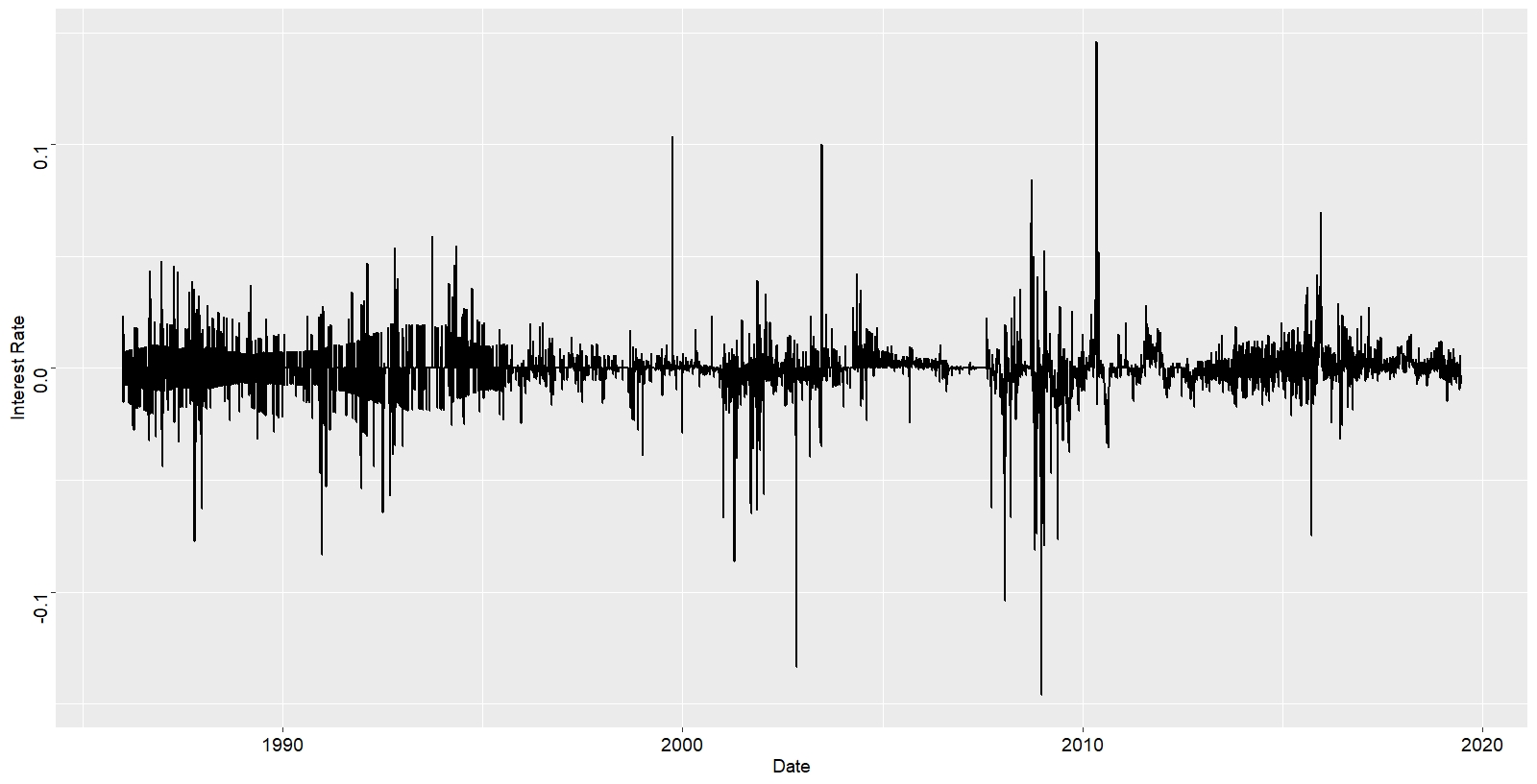
The LIBOR interest rates data obtained from FRED website is known as non-stationary time series data, because the mean, varience, and covariance change over time. If the time series is non-stationary, we can often transform it to stationarity by differencing the data. That is, given the series Z_(t), we create the new series:
Y_(i)=Z_(i) -Z_(i-1)
The differenced data will contain one less point than the original data. Although you can difference the data more than once, one difference is usually sufficient. So to summarize, a stationary time series is the one for which the properties (namely mean, variance and covariance) do not depend on time. Most statistical and financial models and analysis require stationary time series.
The 1 day increment (stationary time series) of USD LIBOR rates can be obtaines in the following manner:
USDON_1D=Delt(USDON, k=1)
USD1M_1D=Delt(USD1M, k=1)
USD3M_1D=Delt(USD3M, k=1)
USD6M_1D=Delt(USD6M, k=1)
USD9M_1D=Delt(USD9M, k=1)
USD12M_1D=Delt(USD12M, k=1)
For example the 3 Month LIBOR interest rate for 1 day increment is:
#plot
C=ggplot() +
  geom_line(data = USD3M_1D, aes(x=index(USD3M_1D), y=USD3M_1D), size=1)+
  ylab("Interest Rate")+
  xlab("Date")+
  theme_gray(base_size = 14)+
  theme(axis.text.y = element_text(size=14, angle = 90 , colour = "black"))+
  theme(axis.text.x = element_text(size=14, colour = 'black'))
print(C)

